No products in the cart.
For permanent magnet materials such as Neodymium-Iron-Boron (NdFeB), our primary objective is to harness their capacity to generate and retain magnetism—the most fundamental functional requirement for any magnetic material. But how, precisely, do we quantify a magnet's ability to generate and preserve this magnetic force? Typically, we employ four key parameters: Residual Induction (Br), Coercivity (Hcb), Intrinsic Coercivity (Hcj), and Maximum Energy Product (BHmax).
To truly grasp the significance of these parameters, one must first understand the concept of the demagnetization curve. Since permanent magnet materials require an initial magnetization process, the resulting magnets must subsequently withstand various adverse factors that could compromise their magnetic properties during actual use; the demagnetization curve serves as an effective tool for comprehensively characterizing the overall performance of a magnet.
The first quadrant is the magnetization curve, the second quadrant is the demagnetization curve, the third quadrant is the demagnetization curve, and the fourth quadrant is the demagnetization curve. The horizontal axis represents the applied magnetic field strength H, and the vertical axis represents the magnetic flux density B and the magnetic polarization J. [Simply put, the magnetic flux density B is the sum of the applied magnetic field and the magnetic field inside the magnet, and the magnetic polarization J is the magnetic field inside the magnet.]
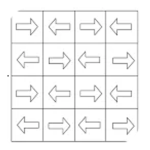
The four magnetic property parameters—remanence, coercivity, intrinsic coercivity, and maximum energy product—are all derived from the demagnetization curve. The J-H demagnetization curve (the curve of the change in magnetic polarization J with the applied magnetic field H), also known as the intrinsic demagnetization curve, and the blue line is called the B-H demagnetization curve (the curve of the change in magnetic flux density B with the applied magnetic field H). We use small squares to represent magnetic domains. A magnetic domain can be understood as a tiny magnet. A magnet is composed of many magnetic domains. The arrows indicate the spontaneous magnetization direction of the domains along the C-axis. For a magnetically neutral permanent magnet (simply put, a magnet that has never been magnetized), most of the magnetic domains are located at the same coordinate but their directions cancel each other out, so they do not exhibit magnetism externally.
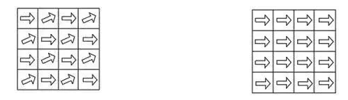
When a magnetic field is applied along the direction of magnetization, the magnetic domains gradually align their c-axes through domain wall displacement and rotation, as illustrated in Figures. This process constitutes the magnetization curve; the value of magnetic polarization intensity exhibited by the magnet at the point of magnetic saturation is termed the saturation magnetic polarization intensity Js.
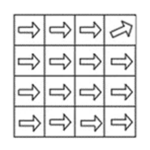
When an external magnetic field is removed after a magnet has reached saturation magnetization, it can be observed—as shown in Figure 4—that the majority of the magnetic domains retain their original orientation; while a small fraction may undergo slight rotation, their predominant alignment remains unchanged. Consequently, both the magnetic induction density and the magnetic polarization of the magnet retain high values. This specific value is termed the *residual magnetic induction density* (Br) or the *residual magnetic polarization* (Jr). Conceptually, it represents the magnetic induction density (B) or magnetic polarization (J) that remains within a magnet after it has been saturated and the external magnetic field has been withdrawn. When the external magnetic field H is zero, Br equals Jr; however, we typically employ Br to characterize this property—what is most commonly referred to simply as *remanence*—measured in units of Gauss (Gs) or Tesla (T).
A higher Br value signifies a greater capacity to retain magnetic induction density, thereby indicating a stronger potential for the material to serve as a high-performance magnetic material.
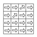
As an external magnetic field is applied in the reverse direction and its magnitude increases, the magnetic domains within the magnet gradually undergo displacement and rotation, as illustrated in Figure. When the magnetic field strength reaches a specific value, the magnetic induction *B* of the magnet drops to zero. Simply put, this occurs because the residual internal magnetic field within the magnet is exactly counterbalanced by the applied external field in the opposite direction. The specific magnetic field strength value at which this occurs is termed the *magnetic induction coercivity* (*Hcb*—also frequently denoted as *bHc*), and its units are Oe or kA/m. The magnetic induction coercivity *Hcb* is closely correlated with the slope of the *J-H* demagnetization curve. If the magnetic domains within the magnet are highly resistant to displacement or rotation—even over short timeframes—the *J-H* curve will appear nearly linear; consequently, the numerical value of *Hcb* will approach *Br* asymptotically. The theoretical upper limit for *Hcb* is *Br* (i.e., *Hcb* = *Br*). This represents an ideal scenario, implying that the magnetic domains exhibit absolutely no tendency to reverse their orientation until the magnitude of the opposing external field numerically equals *Br*. Such a magnet is considered highly stable; specifically, it demonstrates exceptional resistance to demagnetization when subjected to opposing external fields with magnitudes below *Br* relative to its initial state.
As the reverse magnetic field continues to increase, it eventually reaches a critical threshold; at this point, reverse magnetic domains emerge rapidly, causing the magnetic polarization of the magnet to drop swiftly to zero. Simply put, this signifies that the residual magnetic field strength within the magnet has fallen to zero (as illustrated in Figure). The corresponding magnetic field strength value at this juncture is termed the *intrinsic coercivity* (Hcj—sometimes written as jHc), and it is measured in units of Oe or kA/m. Intrinsic coercivity is a physical parameter that quantifies a magnet's inherent resistance to demagnetization; the higher the intrinsic coercivity, the stronger the resistance to demagnetization—or, more precisely, the greater the resistance to *complete* demagnetization. It is crucial here to distinguish between Hcj and Hcb: numerically, when Hcj exceeds Br, the limiting value of Hcb is Br; conversely, when Hcj is numerically less than Br, the limiting value of Hcb is Hcj.
The product of B and H—corresponding to any point on the B-H demagnetization curve—is known as the magnetic energy product. Its maximum value is termed the maximum energy product, denoted as (BH)max. Theoretically, (BH)max = (½ Br)². The maximum energy product serves as a comprehensive metric that balances both residual induction (Br) and intrinsic coercivity (Hcj); its numerical value quantifies the amount of magnetic energy stored within the magnet. It also reflects the initial slope of the J-H curve, and its units are typically expressed in GOe or J/m³.
If the four parameters described above remain difficult to grasp, consider this simple analogy: imagine the magnet as a cup of water. The process of magnetization is akin to heating the water; residual induction (Br) represents the heat retained by the water after the heating source has been removed. Demagnetization, conversely, is analogous to cooling the water down. Hcb represents the specific ambient low temperature at which the external thermal output of the water is completely neutralized—effectively canceling out its internal heat so that no net heat is manifested externally. Finally, Hcj represents the specific ambient low temperature required to reduce the water's internal heat content to absolute zero.
Regarding the aforementioned magnetic parameters, the following points should be noted in practical applications:
For magnets requiring excellent thermal stability, we typically opt to increase the Hcj. This is because, for NdFeB permanent magnets with the same Hcj, the temperature coefficients of coercivity do not vary significantly. The most direct benefit of increasing Hcj is to delay—or ideally prevent—the appearance of the "knee point" in the B-H hysteresis loop. If the requirements for thermal stability are particularly stringent, it is also necessary to consider the Hcb requirements and aim to minimize the slope of the B-H curve in the second quadrant, thereby reducing the magnitude of irreversible magnetic decay in the magnet.