No products in the cart.
Magnetic fields are invisible and intangible; how, then, can we visualize their shapes and map out their direction? Finite Element Simulation offers an excellent method for doing so.
Finite Element Simulation—also known as FEA (Finite Element Analysis)—is a computer-aided technique that employs complex mathematical equations, models, and formulas to simulate real-world physical systems. By utilizing simple, interacting elements (known as "finite elements"), it allows us to approximate a system with infinite variables using a finite number of unknowns. Currently, FEA is widely applied across various fields, including thermal fields, electric fields, magnetic fields, force fields, seepage fields, and acoustic fields. Commonly used software packages for magnetic field simulation include ANSYS, ABAQUS, COMSOL Multiphysics, JMAG-Designer, and EasiMotor.
Mastering simulation software can be relatively challenging. Beyond simply overcoming the technical hurdles of using a new program, one must also understand the specific magnetic parameters associated with the various materials listed in the software's material library. Furthermore, because magnetic field simulation is a relatively niche discipline, the built-in material libraries in almost all software packages often lack comprehensive data for permanent magnets and soft magnetic materials. Consequently, users may frequently need to create new material definitions—a process that involves establishing specific magnetic parameters and demagnetization curves—which requires a thorough understanding of both the materials themselves and the fundamental principles of magnetism.
While specific techniques may vary across different FEA software platforms, this article uses ANSYS as an example to outline the standard procedures for performing finite element simulations of permanent magnets:
1. **Select the Design Type:** ANSYS features numerous design modules. Even within the specialized electromagnetic field suite, there are distinct modules for high-frequency analysis, electric fields, circuit simulation, and magnetostatics. For simulations involving surface magnetism, the "Magnetostatic" module is typically the appropriate choice.
2. **Modeling:** Similar to standard 2D and 3D modeling processes, you must create a geometric representation of the magnet—including its shape, position, and any specific test points—within the software environment. Alternatively, models can be imported directly from external 2D or 3D CAD software packages.
3. **Add Materials:** Properties must be explicitly defined for every material used in the simulation; otherwise, the software will default to treating the material as a vacuum or generate a runtime error. A critical point to note here is that permanent magnets require the explicit definition of a "magnetization direction," which is typically specified relative to the established coordinate system.
4. **Set the Calculation Domain:** Defining an appropriate calculation domain is crucial. If no specific domain is set, the software will default to treating the entire infinite space as the calculation domain. While this approach technically aligns with reality—given that there may indeed be no interfering substances surrounding the magnet—it results in significant computational errors and renders the simulation process extremely time-consuming. 5. **Set Boundary Conditions.** Setting boundaries serves to align with the configuration of the computational domain and reduce the complexity of the problem. Establishing appropriate boundaries can significantly save time during the calculation process. Different boundaries carry distinct physical meanings; typically, for magnetostatic field simulations, we select the "Balloon" boundary condition.
6. **Set Excitation Sources.** When a permanent magnet material is selected, the system automatically applies a magnetostatic excitation source. However, if you need to simulate the magnetic field generated by a coil, you must explicitly add a voltage or current source as the excitation.
7. **Mesh Generation.** Meshing involves discretizing the computational domain into finite elements to construct a mesh structure. The software features a built-in automatic meshing function; generally, the denser the mesh structure, the more accurate the simulation results will be—though this also entails increased computation time.
8. **Configure Solver Settings.** In this section, you can specify parameters such as the allowable error tolerance and the number of calculation steps. The system also provides a set of default settings for convenience.
9. **Define Solution Outputs.** This step determines the specific results you wish to obtain from the simulation—whether you intend to visualize the magnetic flux lines or extract quantitative magnetic field data.
10. **Post-processing.** Once the simulation is complete, you can review various results, including magnetic flux line plots (displayed as either scalar or vector fields), various contour plots, and the specific data and parameters that were designated for simulation at the initial setup stage.
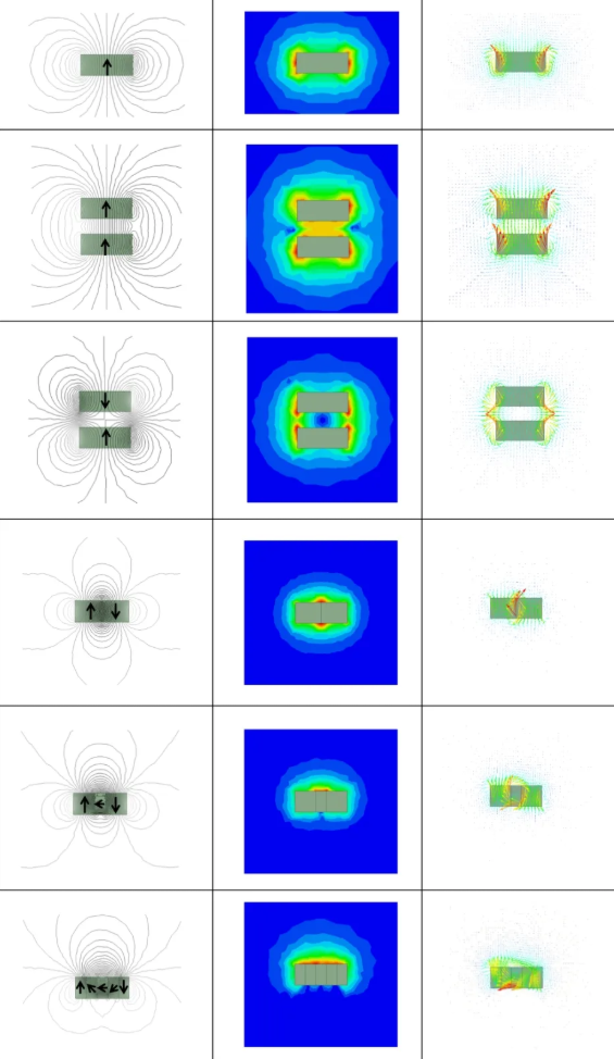
The above outlines the general workflow for using the simulation software. Next, we will present several simulated magnetic field visualizations to help illustrate and facilitate our understanding of magnetic field distributions within different magnetic circuit configurations.