No products in the cart.
Hard magnetic materials, such as neodymium iron boron magnets, have two significant characteristics: first, they can be strongly magnetized under the influence of an external magnetic field; second, they exhibit hysteresis, meaning that the hard magnetic material retains its magnetization state even after the external magnetic field is removed.
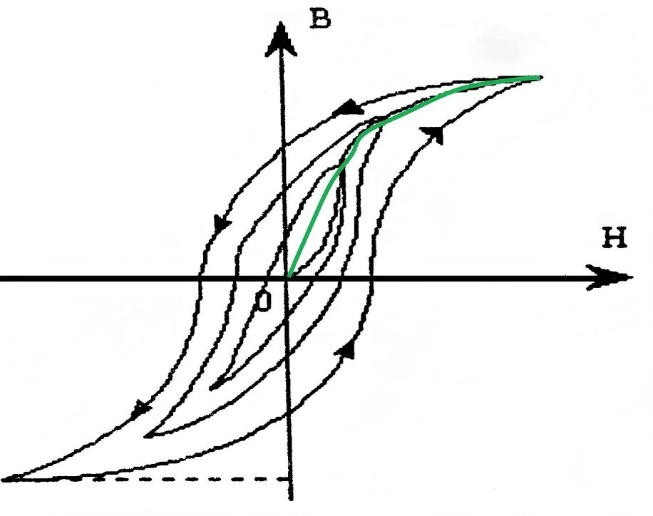
When the magnetic field varies in the following sequence:
Hs → Hc → 0 → -Hc → -Hs → -Hc → 0 → Hc → Hs
the corresponding magnetic induction *B* traces a closed loop along the path S-Hc-S'-Hc-S. This closed loop is known as the **hysteresis loop**.
**Initial Magnetization Curve**
The origin (point 0) indicates that, prior to magnetization, the hard magnetic material is in a magnetically neutral state—that is, *B* = *H* = 0. As the magnetic field *H* begins to increase from zero, the magnetic induction *B* rises slowly, as shown by line segment *oa*. Subsequently, *B* increases rapidly in response to *H*, as shown by segment *ab*. Thereafter, the growth of *B* slows down once again; when *H* reaches the value *Hs*, *B* attains its saturation value, *Bs*. This red curve is referred to as the **initial magnetization curve**.
**Hysteresis**
When the magnetic field is gradually reduced from *Hs* back to zero, the magnetic induction *B* does not retrace the initial magnetization curve back to the "0" point; instead, it decreases along a distinct new curve, *SR*. By comparing line segments *OS* and *SR*, it is evident that while *B* decreases as *H* decreases, the change in *B* lags behind the change in *H*. This phenomenon is termed **hysteresis**. A defining characteristic of hysteresis is that when *H* = 0, *B* does not drop to zero but retains a residual magnetic induction, *Br*.
**Demagnetization Curve**
As the magnetic field is reversed—gradually shifting from point 0 to -*Hc*—the magnetic induction *B* vanishes. This demonstrates that to eliminate residual magnetism, a reverse magnetic field must be applied. The value *Hc* is known as the **coercivity**; its magnitude reflects the magnetic material's ability to retain its residual magnetic state. The purple line segment is referred to as the **demagnetization curve**.
**Basic Magnetization Curve**
By subjecting the same ferromagnetic material to multiple cycles of magnetization using varying magnetic field strengths (*Hm*), a series of hysteresis loops of different sizes can be obtained, as illustrated in the figure below. The curve formed by connecting the vertices of these various hysteresis loops is called the **basic magnetization curve** (or **average magnetization curve**). Although the basic magnetization curve and the initial magnetization curve are not identical, the difference between them is generally negligible; in calculations involving DC magnetic circuits, the magnetization curve utilized is invariably the basic magnetization curve.
The intrinsic magnetic induction produced within a permanent magnet material after it has been magnetized under the influence of an external magnetic field is termed *intrinsic magnetic induction* Bi, also known as *magnetic polarization* J. The curve describing the relationship between this intrinsic magnetic induction Bi or J and the magnetic field strength H serves to characterize the intrinsic magnetic properties of the permanent magnet material; it is referred to as the *intrinsic demagnetization curve*, or simply the *intrinsic curve*.
On the intrinsic demagnetization curve, the magnetic field strength corresponding to the point where the magnetic polarization J equals zero is defined as the *intrinsic coercivity* Hcj.
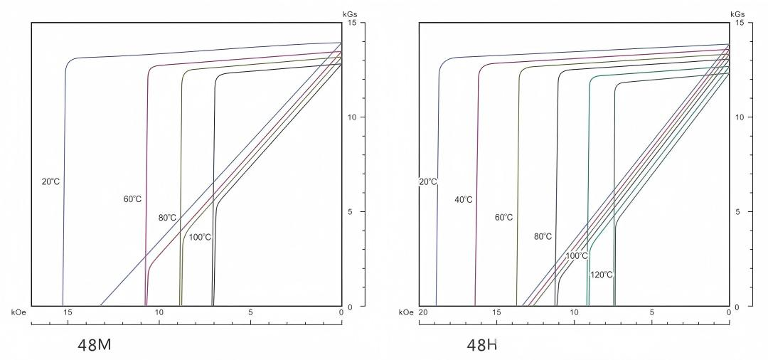
Demagnetization Curves at Various Temperatures
Generally speaking, manufacturers of permanent magnet materials provide demagnetization curves for their various product grades across a range of operating temperatures, as illustrated in the figure below. While this may appear complex, it essentially involves presenting multiple demagnetization curves—along with their corresponding intrinsic curves—on a single graph.